User Help for "Tto®" electrochemical data processing software
Developed by JDMozo for the "Applied Electrochemistry" research group, University of Huelva
|
||||
The Tto electrochemical data processing software begins to develop as a program only for voltammograms representation, because in our Research Laboratory we have many measuring equipment and each one uses a different data file format. So that, if you wanted to compare data from different experiments, it was necessary to dump the data to treatment programs (Excel®, Origin®, SigmaPlot®, ...) by importing them, cleaning all the corresponding header and other additional information available in the file and taking into account the possible difference in the units used for potentials and currents in each type of file.
To facilitate this work we create a program for graph representation (which was autoscale). It must automatically be in charge of the conversion of units, cleaning redundant or unnecessary data and delete headers or others that may be off interest. This seminal simple idea has been growing slowly towards a more powerful program that also allows processing of data contained in the experimental files.
In this help file we pick out a data file of a trace data:
· a data file is a separate file, external to the Tto software , that contains data in a specific format.
· a trace data, or just a trace, is the graphic representation in the Tto software of data in a data file or that derived from a mathematical processing.
The aspect of the main window's Tto software (version 3.0.0.2) not shows any trace of data is the following image:

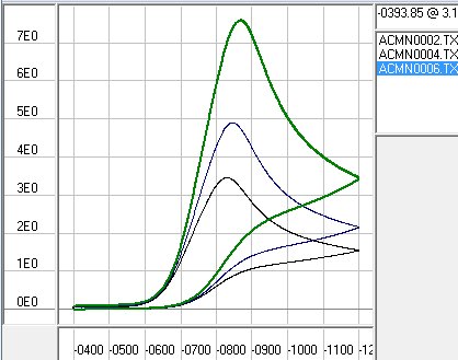
As can be seen, it's simply a menu bar, a graph window and a list indicating the names of trace data being displayed. The location of each zone is much more evident when loading data from one or more files:
X and Y axes are scaled automatically according to the amplitude data shown in the graph window, an excess of 5% of the total size is added on each side for better visualization. The units are set forth in the case of representing voltammograms but can change if you represent cronoamperograms (X ms, and in μA) and absorption spectra (X in nm, and absorption in arbitrary units). In any case the original direction of the axes is growing up and right.
The display of the position coordinates of the cursor indicates the X and Y values corresponding to the position of the cursor when it is within the graph window.
The list of names of traces shown indicates the name of all data traces that the program is showing. If they are derived from data files, the name of the trace coincides with the file that was opened for loading. If you get as a result of treatment, the program assigns a name identifying the trace automatically. On this list you can choose the active trace by simply clicking his name with the mouse, this trace will be the subject of actions outlined in several of menu options.
The data reporting zone is initially empty. It will show the results obtained with the treatments that have numeric character instead of plot.
To facilitate maximum applicability of Tto processing software, it has been developed like a portable application and therefore does not need installation process of any kind. Just copy the executable file Tto.exe on the computer where is used and double-click the icon. It can also be used from a removable drive, flash drive, CD, ...
Sometimes, especially with older operating systems, you must have installed the ActiveX extension comdlg32.ocx used by VisualBasic® programming language. If you first start the Tto software and you receive the follow message "Component comdlg32.ocx or library not found" you can download the extension by clicking here (137KB), copy it directly into the \Windows\System of your computer and try running again the program.
Tto software has been developed for computers running the Windows® operating system. It has worked successfully under Windows 2000®, Windows XP® (SP1, SP2, SP3), Windows Vista® (SP1, SP2) and Windows 7® (32 & 64 bits).
It is necessary to use XP-SP2 compatibility mode in Windows 7 to ensure proper operation. Just set the privilege level to "Run this program as administrator" on the Compatibility tab of the program Properties.
You only need 1MB of disk space and RAM memory requirements depend on the number of traces that are loaded and his size. If memory is insufficient, the program would take more than a few seconds to refresh the graphic window, in this case it is recommended to unload some traces or use a computer with more resources.
The author of the software it’s the sole legal owner. This software is distributed on demand for free, you can use it as is and entirely at your own risk. You can also transfer it to third parties for free but in this case it is recommended that the program is accompanied by an exact copy of this disclaimers and terms of use.
If your use results in the publication of a paper, I would appreciate that this is stated in this publication including a phrase like: "We used the software Tto - ECDPS for ..." and reference as "Mozo, J. D.; Tto Electrochemical Data Processing Software v.4.0, Huelva, SPAIN "
The author is not liable for damages that the use of software may have on your data files. It is recommended to always work with backups.
This is to certify that the software is provided free of viruses and, except for error or omission, works as described in this online help page.
Be sure to use the latest version available by consulting this online help page. If you find any software error or malfunction or even if you want to include some improvement, please consult the author via email.
The following section describes the functions that can be used in each menu option of the program. To easily locate that part of the menu tree we mean at all times, we will use ">" every time we go down a level.
Paragraphs written in this color describes procedures that are not made from any menu item or that can be done directly by pressing a particular keystroke.
 In this
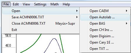
submenu you can specify the name of the file to be loaded to be displayed or
processed in Tto. This option includes several options
that reflect the different data files formats that the program can read,
identified by the name of the measurement equipment that were generated.
If the equipment can
choose between a binary data file format or ASCII (text) files, Tto software will only recognize the latter type.
In this
submenu you can specify the name of the file to be loaded to be displayed or
processed in Tto. This option includes several options
that reflect the different data files formats that the program can read,
identified by the name of the measurement equipment that were generated.
If the equipment can
choose between a binary data file format or ASCII (text) files, Tto software will only recognize the latter type.
Once selected the apparatus that generated the data file, it presents a standard window for disk, directory and name selection on the location of the file. This window allows selecting multiple files by holding down the Shift or Ctrl key while pressing the cursor with different file names. The maximum number of files that can be open simultaneously in Tto software depends on the characteristics of computer used and applications running in it. You should refrain from open more files if you notice that the renewal of the window graph ostensibly slows.
By opening a new file his name appears in the list of names shown traces and it is taken as the active trace.
The file extension automatically showed to select it is in accordance with the approach taken by the equipment manufacturer, in some cases, the file extension indicates the electrochemical technique used to measure and then you can select the appropriate extension in a drop down list .
The extensions that Tto software recognizes are compiled in the following table:
|
Hardware |
Extension |
Commentary |
|
|
CAEM Instrumentation |
SEA1210 |
.DAT |
All techniques |
|
PGA1210 |
.CSV |
Acquired through the Yokogawa DL1520 oscilloscope and stored in ASCII or stored in binary mode and then converted to ASCII with the application wvf2csv.exe |
|
|
.WVF |
Acquired through the Yokogawa DL1520 oscilloscope and stored in binary mode |
||
|
Autolab |
All PGStat |
.OCW |
Cyclic linear sweep voltammetry files |
|
.OEW |
Differential pulse voltammetry files |
||
|
.OXW |
Chronoamperometry files |
||
|
.TXT |
Multi-scan cyclic voltammetry files |
||
|
BAS Inc. |
EpsilonEC |
.DAT |
All techniques. Converted to text from binary files by measurement software |
|
CV 50 |
.TXT |
All techniques. Converted to text from binary files by measurement software |
|
|
BAS100 |
.TXT |
All techniques. Converted to text from binary files by measurement Software |
|
|
CH Instruments |
All potentiostat |
.TXT |
All techniques. Converted to text from binary files by measurement software in any of the possible configurations |
|
Digisim |
.USE |
Simulated cyclic voltammetry files generated by the software |
|
|
.TXT |
Simulated cyclic voltammetry files generated to be exported by the software |
||
|
DropSens |
All potentiostat |
.MTL |
All voltammetry files |
|
.CSV |
Voltammetry files generated to be exported by the software |
||
Gamry |
All potentiostats |
.DTA |
Cyclic voltammetry files |
Scribner Assoc. Inc. |
CorrWare |
.COR |
Cyclic voltammetry files |
| Varian |
Cary 1E |
.CSV |
UV-Vis absorption spectra files compatible with Excel and containing a single spectrum |
|
TXT |
.TXT |
Generated by the Tto software files in a BAS100 compatible format |
|
You can expand the list of currently available data files formats, simply request the author and provide the samples necessary for this.
This action affects the active trace and as a reminder is added to the name of the Save menu title. Using this option can save data from previously opened files or data from changes made on them by mathematical treatment.
Regardless of the original format of the file to save, the Tto software lets you choose a different format (only if the original file was a cyclic voltammetry) so that the generated file can be loaded in the software of a different measurement device that originally used for acquiring them.
Format .USE is the format uses by the Digisym® software as experimental data input. The software will try to adjust a reaction mechanism by compare them with the simulated ones.
Format .SAL is used by ConvIrd.exe application, created to convolute cyclic voltammograms by the "Electrode kinetics and Instrumentation" Research Group at the University of Seville. In a first stage, this software was adopted by Tto for processing data.
When you choose the format to save the active trace data, software shows a window requesting for directory and file name that it will created.
This action affects the active trace to eliminate them among those shown in the graph window. This also affects the list of names of traces shown and the active trace will now be a different from those that remain open.
The Active trace can be closed without using the appropriate menu by pressing <Shift> and <Del> key combinations; this allows to quickly closing a series of consecutive traces.
If the trace to close has not been saved, the Tto software will present a warning before closing and you can cancel the closure of the trace to save them if desired.
This option lets you quit the software. If there are traces that were not stored in files the program informs you before closing and it will be possible to cancel the exit and proceed to save them.
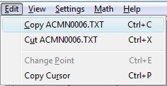 To achieve greater flexibility in
the processing and presentation of data, it is possible to "copy" the
figures for the active trace in the Windows® Clipboard and then
"paste" them in external application having this feature (most of
programs for data processing and graphical representation allowing this form of
import data).
To achieve greater flexibility in
the processing and presentation of data, it is possible to "copy" the
figures for the active trace in the Windows® Clipboard and then
"paste" them in external application having this feature (most of
programs for data processing and graphical representation allowing this form of
import data).
The data is copied without headers or other additions, in two columns contain respectively the values of X and Y in the units used by the Tto program for representation.
The operation of "copy" a trace allows it to remain open in the Tto software and remain as the active trace.
This option "copy" data from the active trace to the clipboard in Windows® in the same way that Copy menu but, unlike what is described in this case, now the trace is closed after copying and active trace becomes another of those that remain open.
This option "paste" data from the clipboard in Windows® to the Tto software and a new active trace is created with them. This is the reverse action of Copy menu and allows you to load data from external processing software or from equipment using ELX application, which loads the adquired data directry to Excel® spreadsheet, such as EL-02.06 potentiostat.
Data should be presented in two columns (variable X on the left and variable Y on the right) and the units must be in accordance with the normally used by the Tto software (potential in mV, current in µA, time in ms). These columns must contain only data (no headers or other information), the numerical format used will be irrelevant.
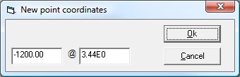 With this menu you
can change the coordinates of a particular point in the active trace through an
input window of numerical values. Initially the window shows the values of the current coordinates of the point to
be edited to provide reference values.
With this menu you
can change the coordinates of a particular point in the active trace through an
input window of numerical values. Initially the window shows the values of the current coordinates of the point to
be edited to provide reference values.
To enable this option menu it is necessary to activate the option View > Set Cursor. So the program can uniquely identify the point to be edited.
This menu provides quick access by pressing simultaneously the keys <Ctrl> + <E>
You can also edit a point, only in its Y coordinate, if you hold down the <Shift> key and right mouse button while moving the cursor over the window graph. The new value of Y that takes the edited point is the same that the cursor when you release the mouse button. This facility allows manual smoothing of the points of the active trace, in a short period of data, in an easy and quickly way.
This option "copies" in the Windows clipboard the coordinates shown in the display of coordinates of the cursor position. This feature facilitates the capture by an external processing software of coordinates corresponding to a particular point on the active trace (e.g. the position of the maximum, zero current potential ...)
This menu provides quick access by pressing simultaneously the keys <Ctrl> + <P>
By activating this option the user can redraw the graph window and the scales of both axes, while respecting the current zoom state. This clears the drawing of "artifacts" that might jeopardize or impair the representation of data open in the software.
This menu provides quick access by pressing the <F4>
View > UnZoom
The user can make zoom on the graph window by dragging the mouse over it while holding down your right mouse button. This action defines (and simultaneously drawn) in the graph a rectangle which has one of the vertex in the position where you press the mouse button and the opposite one at the point where the button is released. This rectangle, plus 5% extra on each side, defines the new scale on the graph to display data.
Using this menu option the user can return to the original graphic scale, in which all data is fully displayed for all open traces.
This menu item is triggered each time you choose a new active trace in the list of names displayed traces.
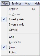 By activating this option the user
can reverse the direction of the X axis scale.
This is particularly interesting to change the display of a reduction
voltammogram and show the style of polarography:
increasing in the negative potential axis to the right.
By activating this option the user
can reverse the direction of the X axis scale.
This is particularly interesting to change the display of a reduction
voltammogram and show the style of polarography:
increasing in the negative potential axis to the right.
When this option is set, it is indicated by a mark left on the submenu displayed. To turn off the option simply rerun the menu.
This menu item is also triggered by double clicking on the X axis scale.
By activating this option the user can invert the Y axis scale. This is particularly interesting to change the display of a reduction voltammogram and show the style of polarography: intensity axis growing up in the negative.
When this option is set, it is indicated by a mark left on the submenu displayed. To turn off the option simply rerun the menu.
This menu item is also triggered by double clicking on the Y axis scale.
This display option facilitates the implementation of Cottrell analysis for data obtained by using cronoamperometry technique. The intensities shown on the Y axis against the inverse of the square root of time data displayed on the X axis. The X-axis transformation will take place in any case, whatever the nature of the data shown in this axis, but of course it will be useful only when the variables represented are related by the Cottrell equation for diffusion-controlled redox processes:
![]()
When this option is set, it is indicated by a mark left on the submenu displayed. To turn off the option simply rerun the menu.
 This option enables the drawing of a
reference grid lines in the graph area to facilitate the visualization of
the traces in a more direct context of relative magnitudes.
This option enables the drawing of a
reference grid lines in the graph area to facilitate the visualization of
the traces in a more direct context of relative magnitudes.
When this option is set, it is indicated by a mark left on the submenu displayed. To turn off the option simply rerun the menu.
View > Cursor Fix
When it is necessary to determine with precision the actual value of a point on the active trace, you can turn on this option. This action causes to display over the active trace a new vertical cursor that follows the mouse pointer (on his vertical) when moving on the graph window but following the intensities of the active trace. When this new cursor is visible, the value of the coordinates displayed on the display of coordinates of the cursor position corresponds to the point of the active trace that is the center of the vertical cursor (the coordinates of a specific point of the trace).
If the active trace has two or more points with the same X coordinate value (e.g. in the case of a cyclic voltammetry trace), the program will search the point of the active trace whose Y value is closest to the mouse pointer position. Just bring the mouse pointer to the wished sweep of the active trace for the vertical cursor is positioned at the points of the trace.
Certain measuring devices generate data files in which the value of the potential (variable X) is digitally measured from analog signal generator rather than being assigned from the control program (digital generation potential). In this case the potentials of the points at the forward and backward sweeps may be slightly different and the vertical cursor can be poorly located even though the mouse pointer is placed near the proper trace. This is not an error and it can be avoided by a digital reconstruction of the trace through resampling points.
This option, along with the following, configures how the traces are displayed in the graph window. By default data represented at traces are consecutively joined by straight lines, but it is possible to combine the display of lines and points as appropriate in each case.
![]()
![]()
![]()
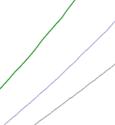
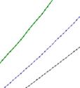
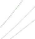
This option, together with the above, lets you configure how the traces are displayed in the graph window. Selecting this option the data represented in traces is drawn as an empty circle centered on the exact coordinates of the point. The radius of the circle depends on the size in pixels of the graphic window and its graphical scale.
Settings> Sens PGA
The CAEM Instrumentation's PGA1210 potentiostat is essentially an analogical system. The digital data files that the Tto program recognizes are those generated by monitoring the analog output signals of potential and current in the Yokogawa DL1520 digital oscilloscope (the work configuration in our laboratory). Both signals must be rearranged and Tto program must know, for the correct representation of voltammogram, which have been the settings of certain operating parameters of the potentiostat.
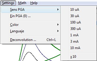 One of the most important measurement parameters with
respect to the output signal corresponding to the intensity level is set at the
potentiostat current follower, which will determine the sensitivity of the
instrument. The
system for monitoring the response current always provides an output signal is
between -10 and 10 V to be registered by the oscilloscope. This voltage signal
will represent a certain amount of current as a function of the scale selected
in the potentiostat rotary switch SENS. indicate the scale selected
by using the dropdown menu PGA Sens at Tto program, you can convert back the voltage file
data in current in the right proportions. If the switch x10 is connected at the
potentiostat, it must be indicated in the Tto
program for a correct interpretation of the sensitivity scale.
One of the most important measurement parameters with
respect to the output signal corresponding to the intensity level is set at the
potentiostat current follower, which will determine the sensitivity of the
instrument. The
system for monitoring the response current always provides an output signal is
between -10 and 10 V to be registered by the oscilloscope. This voltage signal
will represent a certain amount of current as a function of the scale selected
in the potentiostat rotary switch SENS. indicate the scale selected
by using the dropdown menu PGA Sens at Tto program, you can convert back the voltage file
data in current in the right proportions. If the switch x10 is connected at the
potentiostat, it must be indicated in the Tto
program for a correct interpretation of the sensitivity scale.
To other parameter settings refers Settings > Ein PGA (0).
To perform a correct data acquisition it is recommended to set the sensitivity of the oscilloscope channels for signals cover most of the TV screen without clipping. The intensity is read from the Ch1 and Ch2 is for the potential.
Settings > Ein PGA (0)
The CAEM Instrumentation's PGA1210 potentiostat is essentially an analogical system. The digital data files that the Tto program recognizes are those generated by monitoring the analog output signals of potential and current in the Yokogawa DL1520 digital oscilloscope (the work configuration in our laboratory). Both signals must be rearranged and Tto program must know, for the correct representation of voltammogram, which have been the settings of certain operating parameters of the potentiostat.
Regarding the potential output signal, the signal obtained as output and read on the oscilloscope is not that applied to the cell, but it is the generator that produces linear ramps in the potentiostat and will have values between 0 V and the value set to Amp (amplitude sweep) is positive at An mode and negative at Cat mode. The signal applied to the cell is the instrumental addition of this ramp with the continuous potential is set as E.in (initial potential sweep) in the potentiostat multi-turn potentiometers. Tto program must add digitally these values to the voltammogram are conveniently located on the potential scale. To do this, when you select the Settings > Ein PGA menu, opens a window of numerical data entry in which you must specify the initial potential set on the potentiostat, mV (integer with sign). If unchanged, the Tto initial setup program assumes initial potential of 0 mV.
To other parameter settings refers Setup > Sens PGA .
To perform a correct data acquisition is recommended to set the sensitivity of the oscilloscope channels for signals cover most of the TV screen without clipping. The intensity is read from the Ch1 and Ch2 is for the potential.
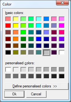 You can customize the look of Tto program regarding the graph window. The three color settings
refer to the active trace, the grid and graphics (the background color of the graph
window and scales on both axes). Selecting any of the three options opens a standard dialog
box in which you can choose the color to apply to the corresponding element.
You can customize the look of Tto program regarding the graph window. The three color settings
refer to the active trace, the grid and graphics (the background color of the graph
window and scales on both axes). Selecting any of the three options opens a standard dialog
box in which you can choose the color to apply to the corresponding element.
Each time you create a new trace in Tto program assigns a color that change automatically in sequence from a selected pre-programmed list into the code itself. This list is designed to optimize each trace individually monitored by well-contrasted colors, both among themselves and against the background. The ability to modify the colors of the traces allows the user to enhance the graphical (or plastic) appearance of a sequence of traces in order to present the results.
For the same reason it may also change the background color of the graphical environment of the program and the grid, if you want it to appear.
Settings > Languaje
This setting configure the languaje used by program Tto in menu options and also in error or advisory alarm. The Tto program can be setting in english or spanish.
This menu selection allows correct the tilt of the active trace that can occur from capacitive current (or load) in a voltammogram or any basis signal that changes smoothly as we move into the coordinate X. The correction is done by subtracting the values of a straight line that fits into an area of active trace where only the basis signal exists.
The modus operandi is as follows:
· At the start of baseline correction Tto program prompts the user a warning window "Select a section of the active trace by 'click' on both ends" and automatically set the option Cursor fix for easy selection of this section.
· The user must choose an area of the active trace as wide as possible where there is only the basis signal.
· The program indicates the position of first point with a cross after you click the left mouse button.
· After clicking a second time at the other end of the selected segment program mark the selected section with a bold and asks for confirmation before proceeding, "Proceed with the selection indicated?"
· If you answered No to this question the transaction will be canceled. If you answer Yes the program calculates the best-fit line to the active trace points included in the section selected. Then subtracted the value calculated by the equation of the line to Y values of all active trace points. The result of this operation is stored and represented in the new trace which is called LBsXXXX where X represent a four digit number that is assigned automatically, increasing to all traces generated by the Tto program as a result of an math operation.
There are mathematical procedures that require for integration or differentiation that the spacing between each pair of points in the variable X is homogeneous in the whole set of data to be processed. Depending on the instrument used for acquired them and/or the conditions of measurement used, a particular data file can comply this or not. In the event that the original data file does not comply with this condition, it can be reconstructed by interpolating the data necessary to meet the target.
Tto program use for this purpose an algorithm based on polynomial interpolation of moving window. This technique involves selecting a certain number of points in the active trace on both sides of the position X where you want to interpolate and least-squares fit a polynomial of certain order. Then calculated the value of this polynomial has at the interpolate point and add the interpolated X and calculated Y values on a new trace to collect the final resample trace. Once this operation changes the value of X to be interpolated and the whole operation is repeated as many times as necessary until the value of X reaches the last point of the trace.
The final result is stored and represented in a new trace which is called RSmpXXXX where X represent a four digit number is assigned automatically, increasing to all traces generated by the Tto program as a result of a processing operation.
Since this involves a calculation of least squares to the new values of Y, an inevitable consequence of resampling the active trace is that it is 'smooth' in some degree. To minimize this effect the width of the moving window should be as small as possible but without this leading to loss of information on the trend of the trace in the neighborhood of the point to be interpolated. Tto program works with a window width of 6 points and the fitted polynomial is of order 2.
In this submenu, encompasses a series of operations that involve the consideration of several traces. These will be combined as appropriate, depending on the selected operation to obtain a new trace with the result of the operation.
Math > Array > Operations > Average
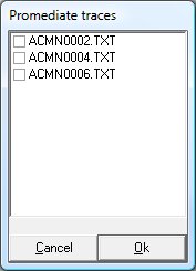 When you select this treatment option, opens a selection window of traces in which the user can specify which traces from those shown in the Tto program will be taken into account to make the average.
To select the traces to average just click the mouse on the box to the left of the trace. It will appear a sign
![]() . Once all the traces was selected to average, the selection will be accepted and the program will calculate the sum of all Y values for each index X and dividing the result by the number of traces selected.
. Once all the traces was selected to average, the selection will be accepted and the program will calculate the sum of all Y values for each index X and dividing the result by the number of traces selected.
Note that to perform this operation does not matter what is the active trace before selecting the menu option since it is not taken into account in a special way to perform the calculation.
To carry out properly this operation it is necessary that theX values of points of each trace are equivalent. This means they must start at the same value, also finished in the same value, and the spacing between data must be equal for all traces. This condition must be achieved relatively easy if the data to be averaged are obtained in different files but using the same test solution and the same measurement conditions. If this were not, traces can be previously prepared by using the resampling option.
The final result is stored and represented in the new trace which is called PromXXXX where X represent a four digit number is assigned automatically, increasing to all traces generated by the Tto program as a result of a processing operation.
Math > Array Operations > Subtract to
This operation is very convenient for the subtraction of traces that contain data from the response of the solvent or other species present in the matrix in which the analyte is dissolved (which is often called background signal) to trace that, in addition to analytical signal sought, has other contributions should be eliminated.
The user must choose how active trace that to which you want to remove the background signal, then select the Subtract to ... operation and, in the trace selection window shown above, to choose those that contain the background signal. Upon acceptance of selection, the program will calculate a new trace in which data of variable Y is calculated as a result of subtraction the Y of the selected traces to the Y of the active trace.
Consideration: should be given the same considerations with respect to the consistency of the traces to be subtracted, which were exposed to the average trace .
The final result is stored and represented in the new trace which is called RstXXXX where X represent a four digit number is assigned automatically, increasing to all traces generated by the Tto program as a result of a processing operation.
This menu is completely analogous to that of average with the exception that in this case, they divide the sum by the number of traces selected.
The utility of this approach is that allows the composition of a complex trace, which the contributions of various analytes from various files in which only measured the signal from one of them. This is of particular interest when peak deconvolution techniques are used: the final stage of the procedure required the reconstruction of the simulated signal and its subsequent comparison with the experimental.
The final result is stored and represented in the new trace which is called SumaXXXX where X represent a four digit number is assigned automatically, increasing to all traces generated by the Tto program as a result of a processing operation.
Tto program allows applying a digital filtering algorithm based on the Savitzky-Golay described in the article "Smoothing and Differentiation of data by simplified least squares procedures" Analytical Chemistry, 1964, 36 (8) , pp 1627-1639. The implementation of this algorithm is equivalent to using a low-pass filter that removes higher frequency components of the signal. The program allows you to choose filter orders n = 5, 7, 9 and 11.
 This algorithm apply to each point of the active trace a polynomial fit of order (n - 1)/2 to n points around to the filtrate. The polynomial coefficients are not calculated because they are constant characteristics of the filter. The ultimate effect of implementing the routine is similar to a mobile weighted average to Y coordinate of each point of the trace.
Like when you apply an instrumental filter to an analytical signal, we must take in mind that the signal passing through the filter can distort to some extent the signal information, because the mission of a filter is to remove certain range of frequency components of the filtered signal. This degradation of the filtered signal will be greater the more effective the filter used, so we must be careful with the use of any filter.
When using a digital filter that consideration should be taken into account as well. However, at the Tto program user can observes degradation suffered by the original signal to be filtered since it preserves the original signal and this can be compared with that obtained by filtering. The filtered signal should be free of sharp peaks (corresponding to high frequency noise), but must follow, in general, the behavior of the original signal. Thus, it is easy to decide which the most suitable filter is.
The final result is stored and represented in the new trace which is called FltXXXX where X represent a four digit number is assigned automatically, increasing to all traces generated by the Tto program as a result of a processing operation.
Math > Deconvolution
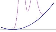
 The Tto program allows deconvolute peaks at complex trace where the analytical signals are symmetrical, obtained by techniques such as differential voltammetry, chromatography, etc...
The deconvolution allows, through a complex mathematical process, to extract information on the various components that make up the response of a measurement process. Tto program allows the analysis of experimental response signal, which consists of the superposition of several simple signals, in a simple way thanks to the graphical approach to the problem.
The calculation procedure can be summarized in the following steps:
· Propose many Gaussian or Laurentian functions as are necessary to compose the experimental trace.
· Propose, if necessary, a baseline that takes into account the background signal of the experimental trace.
· Select the experimental trace as active trace.
· Adjust the proposed theoretical functions to experimental.
Each of these steps is explained in detail below.
Math > Deconvolution > New Baseline
You can create a new trace whose points are calculated by a polynomial equation of second order. This trace should be as close as possible to the background signal from a trace containing experimental data with the intention of being used for adjusting the signal.
To calculate the polynomial coefficients, the Tto program prompts you to enter the coordinates of three points that satisfy his equation.
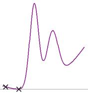 The statement of the points of the polynomial is done graphically by clicking on the graphic window for three consecutive times. Each time you click, the program marks the spot with an X to record that has been selected one of the points and to place which is the place regarding the traces that are showing. Having been set the third point, coordinates are processed, the polynomial coefficients
 are calculated by using the Lagrange interpolation method and a new trace is create with graphical
representation of the function obtained, which is called LBP2XXXX where X represents a four-digit number assigned automatically, increasing to all traces generated by the Tto program as a result of a processing operation.
are calculated by using the Lagrange interpolation method and a new trace is create with graphical
representation of the function obtained, which is called LBP2XXXX where X represents a four-digit number assigned automatically, increasing to all traces generated by the Tto program as a result of a processing operation.
The Lagrange interpolation method, or rather the form of Lagrange polynomial interpolation, was developed by E. Waring in 1779 and L. Euler in 1783 and they are examples of programming routines for different languages in ALGLIB Open Source.
The activation status of the View > Cursor fix determines whether the points chosen for the calculation will be on the active trace or at any point in the graphic window. Configure the program according to your needs.
Math > Deconvolution > New Gaussian
You can create a new trace whose points are calculated by Gauss equation. This trace should be as close as possible to any part of a trace that represent experimental data and containing analytical information intended to be used for adjusting the signal.
![]()
The shape of the Gaussian function used is indicated in the above equation. To obtain the coefficients of the function, the Tto program prompts you to enter the coordinates of two points representing:
1. the maximum intensity (which determines both the maximum of the function (A) and maximum's X coordinate (B)) and
2. the peak full-width at half maximum intensity (FWHM) (determined by the X position of second point (C) being its Y coordinate irrelevant). Choose this point to the right or left of the first has no effect on the calculated function.
The statement of the points is done by clicking on the graphic window twice in a row. Each time you click, the program marks the spot with an X to record that has been selected one of the points and to place which is the place regarding the traces that are showing. Having been set the second point, coordinates are processed, coefficients of the function are calculated and a new trace is created, with graphical representation of the function obtained, which is called GausXXXX where X represent a four digit number assigned automatically, increasing to all traces generated by the Tto program as a result of a processing operation.
Math > Deconvolution > New Lorentzian
You can create a new trace whose points are calculated by Lorentz equation. This trace should be as close as possible to any part of a trace that represent experimental data and containing analytical information intended to be used for adjusting the signal.
 The shape of the Lorentzian
function used is indicated in the above equation. To obtain the coefficients of the function, the Tto program prompts you to enter the coordinates of two points representing:
The shape of the Lorentzian
function used is indicated in the above equation. To obtain the coefficients of the function, the Tto program prompts you to enter the coordinates of two points representing:
1. the maximum intensity (which determines both the maximum of the function (A) and maximum's X coordinate (B)) and
2. the peak full-width at half maximum intensity (FWHM) (determined by the X position of second point (C) being its Y coordinate irrelevant). Choose this point to the right or left of the first has no effect on the calculated function.
The statement of the points is done by clicking on the graphic window twice in a row. Each time you click, the program marks the spot with an X to record that has been selected one of the points and to place which is the place regarding the traces that are showing. Having been set the second point, coordinates are processed, coefficients of the function are calculated and a new trace is created, with graphical representation of the function obtained, which is called LorzXXXX where X represent a four digit number assigned automatically, increasing to all traces generated by the Tto program as a result of a processing operation.
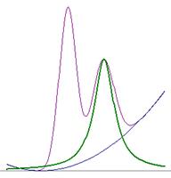
Once created the traces that you want to adjust to the experimental data, they can be added to assess the degree of accuracy achieved in the first attempt. How you use this option has already been explained earlier in the Math > Array Operations > Add menu.
Math > Deconvolución > Ajustar a
To refine the initial adjust, Tto program uses the Levenberg-Marquardt algorithm, K. Levenberg " A Method for the Solution of Certain Non-Linear Problems in Least Squares " The Quarterly of Applied Mathematics, 1944, 2 , pp 164-168 and D. Marquardt "An Algorithm for Least-Squares Estimation of Nonlinear Parameters" SIAM Journal on Applied Mathematics, 1963, 11 , pp 431-441, for multi-parameter least squares fit of the sum of multiple traces to that is selected as active trace.
 The Levenber-Marquardt
algorithm is a fitting system which converges rapidly and has high reliability. The Tto program allows iterations up to 10,000 or to achieve convergence with a cumulative tolerance between the calculated points and the goal of 2 x 10-16. The fit affects the values of three parameters for each trace considered, these parameters are recalculated for each iteration, and
with them the points of the resulting traces are compared with the active trace to check the degree of convergence. There are
examples of programming routines of this algorithm for different languages in ALGLIB Open
Source.
The Levenber-Marquardt
algorithm is a fitting system which converges rapidly and has high reliability. The Tto program allows iterations up to 10,000 or to achieve convergence with a cumulative tolerance between the calculated points and the goal of 2 x 10-16. The fit affects the values of three parameters for each trace considered, these parameters are recalculated for each iteration, and
with them the points of the resulting traces are compared with the active trace to check the degree of convergence. There are
examples of programming routines of this algorithm for different languages in ALGLIB Open
Source.
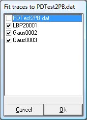
To select the traces to be considered in the fitting, the Tto program presents a window selection
with all existing
traces. You should select
those that wish to use (except the active trace to act as a target in the fitting). To select the traces just click the mouse on the box to the left of the trace, it will appear a sign
![]() . Once indicated all the traces that they will use to fit, the selection must be accepted and the program
will start calculating the sum of all Y values
for each index X and approximating this sum to the active trace.
. Once indicated all the traces that they will use to fit, the selection must be accepted and the program
will start calculating the sum of all Y values
for each index X and approximating this sum to the active trace.
As the calculation proceeds, in the data reporting zone shows the number of iterations performed. When the process have been completed, the final values of optimized parameters are showed in the same data reporting zone, redraw the traces selected for the calculation according to the final results and creates a new trace with the resulting data to add them which is called FitXXXX where X represent a four digit number is assigned automatically, increasing to all traces generated by the Tto program as a result of a processing operation.
In this submenu, a series of operations involving the active trace and a scalar number to be applied on each and every one points of the trace are included. The result of the operation would lead to a new trace.
Math > Scalar Operations > Multiply by nr.
The possibility of multiplying the values of the Y coordinate of each point of a trace permits to adjust measurements on different computers so they can be compared among themselves. For example, voltammograms carried on working electrodes with different area, spectra made in sample cells with different optical path, etc...
 After selecting the menu option, it provides an input window where you specify the value (real) of the
multiplying factor to be applied in the operation. You can enter both positive and negative values. The decimal separator can be either a dot "." or a comma "," as the Tto program is capable of processing both.
After selecting the menu option, it provides an input window where you specify the value (real) of the
multiplying factor to be applied in the operation. You can enter both positive and negative values. The decimal separator can be either a dot "." or a comma "," as the Tto program is capable of processing both.
After being typed the value you click on the OK button or press the <Enter> (<Intro>, <
![]() >),
calculated the new Y coordinates and creating a new trace, which is called MultXXXX where X representing a four digit number is assigned automatically, increasing to all traces generated by the Tto program as a result of a processing operation.
>),
calculated the new Y coordinates and creating a new trace, which is called MultXXXX where X representing a four digit number is assigned automatically, increasing to all traces generated by the Tto program as a result of a processing operation.
Math > Scalar Operations > Add nr. to X
Adding a constant to the values of the X coordinate of each point of a trace can move the trace along the horizontal axis for better comparison of measurements in different conditions. For example, voltammograms made against different reference electrodes, etc ...
After selecting the menu option, it provides an input window where you specify the value (real) number to be added (with its sign) to the X coordinate of each point. You can enter both positive and negative values. The decimal separator can be either a dot "." or a comma "," as the Ttoprogram is capable of processing both.
After being typed the value you click on the OK button or press the <Enter> (<Intro>, <
![]() >),
calculated the new X coordinates and creating a new trace, which is called OffxXXXX where X representing a four digit number is assigned automatically, increasing to all traces generated by the Tto program as a result of a processing operation.
>),
calculated the new X coordinates and creating a new trace, which is called OffxXXXX where X representing a four digit number is assigned automatically, increasing to all traces generated by the Tto program as a result of a processing operation.
Math > Scalar Operations > Add nr. to Y
 Adding a constant to the values of the Y coordinate of each point of a trace can move the trace along the vertical axis for better comparison of measurements in different conditions, i.e., to change uniformly the baseline of the trace.
After selecting the menu option, it provides an input window where you specify the value (real) number to be added (with its sign) to the Y coordinate of each point. You can enter both positive and negative values. The decimal separator can be either a dot "." or a comma "," as the Tto program is capable of processing both.
After being typed the value you click on the OK button or press the <Enter> (<Intro>, <
![]() >),
calculated the new Y coordinates and creating a new trace, which is called OffYXXXX where X representing a four digit number is assigned automatically, increasing to all traces generated by the Tto program as a result of a processing operation.
>),
calculated the new Y coordinates and creating a new trace, which is called OffYXXXX where X representing a four digit number is assigned automatically, increasing to all traces generated by the Tto program as a result of a processing operation.
The choice of this treatment is only active when you select the viewing option View > Cottrell. This treatment involves adjusting by least squares a line to a series of interrelated data by using the Cottrell equation. According to this equation, the slope of the fitted line has information on the number of electrons exchanged per mole of reacted species (n), the electrode area (A), the concentration of electro-active species (Co) and the diffusion coefficient of the species (D). If these parameters are known, or can be calculated using other techniques, we can calculate that we do not know.
![]()
After selecting this treatment option on the menu, the program prompts you to select the area of the active trace to be used for treatment. This selection is done by clicking the two points that define the area of the trace. Once you have confirmed the desired selection, Tto program performs statistical calculation, draw the line of best fit and show the parameters in the data reporting zone.
 In this submenu are included two ways to implement the convolution, also called half-integration or half-differentiation, described by KB Oldham in his article "Convolution: a general electrochemical procedure Implemented by a universal algorithm", Analytical Chemistry, 1986, 58, pp 2296 - 2300. This treatment transforms a cyclic voltammogram so it is possible to extract information about the reaction mechanism and kinetic and/or thermodynamic
parameters in a more simple and, above all, reliable because it takes into account all the data in voltammogram and not only the maxima of these waves. Also, instead of being required a set of measurements made at various scan rates, just process a single voltammogram to get results.
In this submenu are included two ways to implement the convolution, also called half-integration or half-differentiation, described by KB Oldham in his article "Convolution: a general electrochemical procedure Implemented by a universal algorithm", Analytical Chemistry, 1986, 58, pp 2296 - 2300. This treatment transforms a cyclic voltammogram so it is possible to extract information about the reaction mechanism and kinetic and/or thermodynamic
parameters in a more simple and, above all, reliable because it takes into account all the data in voltammogram and not only the maxima of these waves. Also, instead of being required a set of measurements made at various scan rates, just process a single voltammogram to get results.
Convolution transform the intensity data in a voltammogram in convoluted intensity data with the following operation, where the asterisk represents the convolution operation between the voltammogram and the convolution function, g(t), which depends on the symmetry of the electrode and type of mechanism by reaction occurs:
![]()
For the simplest case, a simple electronic transference on semi-infinite flat electrode geometry, the convoluted intensity is obtained from the operation:
![]()
It is important to note that in order to make the convolution of a voltammogram, it must have current data at regular intervals of time (or potential). If this is not true in the original file, trace should be resampled before by option Math > Resample each mV
 Math > Convolution >
Using ConvIrd.exe
Math > Convolution >
Using ConvIrd.exe
ConvIrd is an external application to Tto program that was developed by the Research Group "Electrode kinetics and Instrumentation" at the University of Seville for the transformation of cyclic voltammograms by convolution technique. It is a DOS application that is applied to a data file whose header includes the parameters that the program needs for its calculation. Tto program facilitates the creation of this file by using a parameter's input window that must be properly completed. The meanings of the parameters are:
Electrode: Parameters related to its shape and size
- Symmetry (electrode shape): can be indicated Flat (disc electrode) and Spherical (drop electrode)
- Radius (electrode size): indicates a default value, should be indicated for the electrode used to obtain the data file to be treated. Its value is only relevant if the symmetry is spherical.
Other parameters:
- Sweep rate: This parameter can reflect the value read from the data file's header, or a default value that should be modified to achieve a consistent result.
- Diffusion Coeff: provides a default value that corresponds to the usual organic molecules in solvents of medium polarity. Its value is only relevant if the symmetry is spherical.
Kinetic fitting: ConvIrd program also performs convolution calculations suitable for EC-type mechanisms. The calculation of the rate constant of step C (the value of K) is obtained by using tentative values of K in the convolution equation and trying the convoluted current to backward sweep end is zero. ConvIrd finds the value of this constant by using an iterative calculation.
- K Initial value: K value used as starting point for the iterative calculation.
- Regression points nr: number of points in the end of backward sweep that ConvIrd used to verify that the convoluted current is zero.
- Maximum iteration nr: to avoid a no convergence, ConvIrd stop the calculation if it reaches the iterations number listed here.
Once these data, Tto program create a temporary file which is used by ConvIrd for calculations as input. ConvIrd> then generates an output file that contains information about the calculation process and convoluted intensity data. Tto program will read this output file and create two new traces with its content, one that represents the convoluted intensities for a single electronic transference (E) and another with the convoluted intensities taking into account the coupled kinetic stage (C). Also it indicates the number of performed iterations, the final value of K obtained and the fit average deviation in the data reporting zone. The new traces with the resulting data are called respectively CinXXXX and ConvXXXX where X represent a four digit number is assigned automatically, increasing to all traces generated by the Tto program as a result of a processing operation.
To use this calculation option, it must have ConvIrd.exe program (not supplied with Tto) and it must be located in the root directory of the boot drive (C: \)
Math > Convolution > Using inner routine
 To avoid the need for ConvIrd program, Tto also includes its own convolution routine. Similarly to
the above, it should indicate the experimental parameters with that voltammetric data were acquired for the result of the convolution make sense. When you select this menu option a window configuration opens to be completed.
To avoid the need for ConvIrd program, Tto also includes its own convolution routine. Similarly to
the above, it should indicate the experimental parameters with that voltammetric data were acquired for the result of the convolution make sense. When you select this menu option a window configuration opens to be completed.
Depending on the selected symmetry, the parameters for the electrode radius and the diffusion coefficient will be active or not.
If you check the homogeneous kinetics option, you are also asked to list the value of K homogeneous, necessary for convolution function. Unlike ConvIrd, now only is performed the calculation of a convoluted voltammogram whose results are shown. It is the responsibility of the user to adjust the value of K to obtain a homogeneous kinetic convoluted voltammogram similar to the not-kinetic convolution. At this time there will be the real value of K.
The trace with the resulting data set is called ConvXXXX where X represent a four digit number is assigned automatically, increasing to all traces generated by the Tto program as a result of a processing operation.
 Given the great utility, for analytical purposes, that has to know the value of the charge circulated during a redox process or, in general, the area under the curve of an analytical signal, the Tto program incorporates this facility in a very flexible and simple way.
It should be used always a trace which has been corrected from its baseline to avoid contributions to the area that do not correspond to analytical information. The way that the baseline correction should be made is the responsibility of the user, and depends on the characteristics of signal processing. However, it is recalled that the Tto program has do it in three different ways: by option Math > Correct baseline for a linear correction, by option Math > Array Operations > Subtract for the subtraction of a trace containing the base signal, and through option Math > Deconvolution > New baseline for creating a second order baseline, followed by Math > Array Operations > Subtract to subtract the previously established baseline.
The fragment of the active trace to be integrated also depends on the characteristics of the signal: if it is symmetric (Gaussian) tends to integrate the whole signal, if it is asymmetrical (similar to the voltammetric or chromatographic) usually integrate only the first half thereof.
In any case, the Tto program also offers complete freedom regarding the limits of integration. The user can graphically select them by clicking on both ends of the area to integrate over the active trace. After selecting the first point the Tto program mark them with a cross to indicate that it has been selected, and for the user consider his position by stating the second limit. The selection of the second limit in turn activates a request for confirmation, and then start calculating the area by the sum of the areas of trapezoids inscribed under each pair of points included in the selected range. The absolute value of the total area obtained is shown in the data reporting zone, and the area processed is represented graphically.
Starts the default Web browser and submit this document. If this operation fails, a warning window is popped up indicating the URL where you can find this document.
Version
1.0
Revision #1:
· Ability to read .TXT files is included
· Ability to change color of traces, grid and background is included
· Zoom error correction to consider inverted axis possibilities is fixed
· Cursor fix menu option is moved to View menu
Revision #2:
· Error on cumulative treatment is fixed
· Error on ticY calculation for decimal progress (scale smaller than an integer) is fixed
Revision #3:
· Error on minimize window is fixed
· Savitzky-Golay numerical filter is included
· Cursor height calculation in terms of intensity scale is fixed
Revision #4:
· Baseline correction is included
Revision #5:
· Trace subtraction (if several traces are selected only the last is subtracted) is included
· Active trace name in menu options is included
Revision #6:
· Edit>Copy/Cut is included
· Fixed graphical scale when all traces are closed
· Fixed select active trace when the first trace is closed
Revision #7:
· Load .DAT cronoamperometry files is fixed
· Ask before close unsaved file
· Cottrell view for cronoamperometry is included
· Cottrell analysis (i = A / sqr(t) + B) is included
Revision #8:
· Reading of .CSV Cary files saved as spreadsheet is included
· Gauss and Lorentz functions to deconvolution is included
Revision #9:
· Reading .ocw Autolab files (cyclic voltammetry) is included
· Reading .oew Autolab files (differential voltammetry) is included
· Reading .oxw Autolab files (cronoamperometry) is included
· Multiply Y axis by nr. Is included
· Add offset to X axis is included
Revision #10:
· Reading of Autolab files is fixed by correcting potential data
Version 2.0
Revision #0:
· Convolution through C:\Convird.exe is included
· Error in multiple file loading (only W98) is fixed
· .DAT and .SAL format on save files are included
Revision #1:
· Display of the position coordinates is changed to x @ y
· Add/average/subtract inconsistent files is facilitates
· Frees memory by unload traces
Revision #2:
· Reading files from remote location (network) is included
Revision #3:
· Shutdown on reading file error is fixed
· Include trace resampling for potentials at .OCW Autolab files
· Units of electrode radius are fixed
Revision #4:
· Active trace is indicate in resample menu option
· Properties of traces are dragged to derived ones
· Reading of .DAT EpsilonEC files (only CV) is included
· Reading of .TXT Bas100 files is included
Version
2.1
Revision #0:
· Convolution by own routine is included for several symmetry (first approximation)
Revision #1:
· Error on labeling resample results is fixed
· Error on resample turnover detection is fixed
· Hourglass pointer is showed on convolution by own routine
· Lines and/or points data representation in included
· Refresh graph without changes zoom is included (F4)
· Edit point Y value by drag and drop is included (Shift + cursor fix)
· Edit point position by input window is included
· Save ConvIrd .DAT file is included
· Save Autolab .OCW file is included
Version
2.2
Revision #0:
· Resampling by mobile window interpolation method is included
· Calculation error on convolution is fixed (double precision variables to avoid digital noise)
Revision #1:
· .TXT output format is adapted to match Bas100
· Reading error on .OCW saved files is fixed
· Properties of new traces are dragged from active trace
· Fast convolution routine is include in own routine
· Ask for scan rate on save .TXT files if this data doesn't exist
Revision #2:
· Error on save .TXT Bas100 files with resampled data is fixed
Revision #3:
· Reading .DAT Epsilon EC files (VPD and CA) is included
Version
3.0
Revision #0:
· Lagrange polynomial interpolation is include to solve second order polynomial baseline
· Levenbert-Marquard signal deconvolution algorithm is included
· Deconvolution includes Gaussian, Lorenztian and second order polynomial baseline
Revision #1:
· Open ASCII (*.csv) data file from Yokogawa oscilloscope is included
Revision #2:
· Copy pointer position on Windows clipboard
· Load error on BAS100 files whose scan rate is V/sec or µV/sec is fixed
Revision #3:
· Hyperlink to www.uhu.es/giea/ayuda.htm help file is included
Revision #4:
· Open .txt and .use Digisim exported data files is included
· Shortcut keystrokes to Copy and Cut are included
· Open .txt BAS CV-50W data files is included
· Open .txt CHI data file is included
· Tree menu structure File > Open > is optimized
· Format of .txt saved files is modified to match BAS100 format
Revision #5:
· Area numerical calculation is included
· Polynomial baseline can be calculated using anywhere points or trace points depending on the Cursor Fix state
Revision #6: (Nov 2010)
· Settings window to configure mean square multi-parametric L-M fitting is included
· Exit program with red X upper-right corner is disabled
Revision #7: (Feb 2011)
· Load Cary 1E data files is corrected (it can be load .csv files regardless of the language settings of the computer where they're generate)
· Numerical filter order 9 and 11 are included
Revision #8: (Mar 2011)
· Load DCPA Epsilon files is included and other techniques are forbidden to prevent errors
Revision #9: (Apr 2011)
· Distinguish Cary files containing spectra (Abs vs. wavelength) from which contain kinetics (Abs vs. t(ms))
· Errors on X axis scale calculation are fixed (ticX evaluation and X index greater than integer)
Version 4.0
Revision #0: (Apr 2011)
· Menu tree and messages box translated to english (bilingual software)
Revision #1: (Jul 2011)
· Load DropSens files is included (*.mtl & *.csv)
Revision #2: (Oct 2011)
· Load SPTB BAS100 files is included and other techniques are forbiden to prevent errors
Revisión #3: (Feb 2012)
· Two columns data load from Window's Clipboard is included (CV data read from EL-02.06 potentiostat and ELX software)
· Load DPV BAS100 files is included