Inicie su sesión para modificar los apuntes, usar los foros, etc. Si no es usuario de la web, regístrese.

Contenidos licenciados 
![]()
Revisión de Resuelto. Ejercicio 2 de diciembre del 2008. (3.5 puntos) de 15 January, 2011 - 15:25
25 June, 2009 - 14:09 — oscaralonso.idarraga
 Versión para imprimir
Dada la siguiente ecuación diferencial:
$$\dfrac{\partial^3 y(t)}{\partial t^3}+4\dfrac{\partial^2 y(t)}{\partial t^2}+5\dfrac{\partial y(t)}{\partial t}+y(t)+\sin(y(t))-r(t)=0$$
1) Obtener un modelo de estado que represente el sistema no lineal.
2) Obtener un modelo de estado lineal del sistema suponiendo que éste opera en las cercanías del punto y(t)=0
3) Simular durante 20 segundos tanto el sistema lineal como el sistema no lineal, si se toma como punto inicial el origen, para r(t)=1 y r(t)=5, comentando los resultados de la simulación.
Deberá crear una función en un archivo M que describa el sistema no lineal, para poder simularlo mediante la instrucción ode 45
APARTADO 1.
Como la mayor derivada es 3, sabemos que N=3.
\[
\begin{array}{l}
x1 = y(t) \\
\mathop {x1}\limits^ \bullet = \mathop y\limits^ \bullet (t) = x2 \\
\mathop x\limits^ \bullet 2 = \mathop y\limits^{ \bullet \bullet } (t) = x3 \\
\mathop x\limits^ \bullet 3 = \\
\end{array}
\]
Despejamos de la ecuación \[\mathop x\limits^ \bullet 3\] pero primero reemplazamos los nombres
\[
\begin{array}{l}
\mathop x\limits^ \bullet 3 + 4x3 + 5x2 + x1 + sen(x1) - r(t) = 0 \\
\mathop x\limits^ \bullet 3 = - 4x3 - 5x2 - x1 - sen(x1) + r(t) \\
\end{array}
\]
Por tanto el modelo de estado seria:
\[
\begin{array}{l}
\mathop {x1}\limits^ \bullet = x2 \\
\mathop x\limits^ \bullet 2 = x3 \\
\mathop x\limits^ \bullet 3 = - 4x3 - 5x2 - x1 - sen(x1) + r(t) \\
\end{array}
\]
Y la sálida será:
\[
y(t) = x1
\]
APARTADO 2.
\[
\frac{{\partial ^3 y(t)}}{{\partial t^3 }} + 4\frac{{\partial ^2 y(t)}}{{\partial t^2 }} + 5\frac{{\partial y(t)}}{{\partial t}} + y(t) + sen(y(t)) - r(t) = 0
\]
Como \[
sen(y(t))
\]
es no lineal, lo linealizamos por medio del polinomio de Taylor.
\[
\begin{array}{l}
sen(y(t)) \cong sen(y_0 (t)) + \left. {\frac{{\partial sen(y(t))}}{{\partial t}}} \right|_{x_0 } *\frac{{(y - y_0 )}}{1} + ... \\
sen(y(t)) \cong sen(y_0 (t)) + \cos y(t)*(y - y_0 ) + ... \\
\end{array}
\]
Estudiamos el caso para \[
y_0 (t) = 0
\]
Que reemplazandolo será
\[
\begin{array}{l}
sen(y(t)) \cong 0 + 1(y - 0) \\
sen(y(t)) \cong y \\
\end{array}
\]
Por tanto la ecuación quedaría
\[
\begin{array}{l}
\frac{{\partial ^3 y(t)}}{{\partial t^3 }} + 4\frac{{\partial ^2 y(t)}}{{\partial t^2 }} + 5\frac{{\partial y(t)}}{{\partial t}} + y(t) + y(t) - r(t) = 0 \\
\frac{{\partial ^3 y(t)}}{{\partial t^3 }} + 4\frac{{\partial ^2 y(t)}}{{\partial t^2 }} + 5\frac{{\partial y(t)}}{{\partial t}} + 2y(t) - r(t) = 0 \\
\end{array}
\]
Ahora convertimos la ecuación en modelo de estados
Como la mayor derivada es 3, sabemos que N=3.
\[
\begin{array}{l}
x1 = y(t) \\
\mathop {x1}\limits^ \bullet = \mathop y\limits^ \bullet (t) = x2 \\
\mathop x\limits^ \bullet 2 = \mathop y\limits^{ \bullet \bullet } (t) = x3 \\
\end{array}
\]
Despejamos de la ecuación \[\mathop x\limits^ \bullet 3\] pero primero reemplazamos los nombres
\[
\begin{array}{l}
\mathop x\limits^ \bullet 3 + 4x3 + 5x2 + 2x1 - r(t) = 0 \\
\mathop x\limits^ \bullet 3 = - 4x3 - 5x2 - 2x1 + r(t) \\
\end{array}
\]
Por tanto el modelo de estado seria:
\[
\begin{array}{l}
\mathop {x1}\limits^ \bullet = x2 \\
\mathop x\limits^ \bullet 2 = x3 \\
\mathop x\limits^ \bullet 3 = - 4x3 - 5x2 - 2x1 + r(t) \\
\end{array}
\]
Y la sálida será:
\[
y(t) = x1
\]
Representado de forma matricial seria.
\[
\left[ {\begin{array}{*{20}c}
{\mathop {x1}\limits^ \bullet } \\
{\mathop {x2}\limits^ \bullet } \\
{\mathop {x3}\limits^ \bullet } \\
\end{array}} \right] = \left[ {\begin{array}{*{20}c}
0 & 1 & 0 \\
0 & 0 & 1 \\
{ - 2} & { - 5} & { - 4} \\
\end{array}} \right]*\left[ {\begin{array}{*{20}c}
{\mathop {x1}\limits^{} } \\
{\mathop {x2}\limits^{} } \\
{\mathop {x3}\limits^{} } \\
\end{array}} \right] + \left[ {\begin{array}{*{20}c}
0 \\
0 \\
1 \\
\end{array}} \right]*r(t)
\]
Y la sálida será:
\[
\left[ {y(t)} \right] = \left[ {\begin{array}{*{20}c}
1 & 0 & 0 \\
\end{array}} \right]*\left[ {\begin{array}{*{20}c}
{x1} \\
{x2} \\
{x3} \\
\end{array}} \right] + \left[ 0 \right]*r(t)
\]
APARTADO 3.
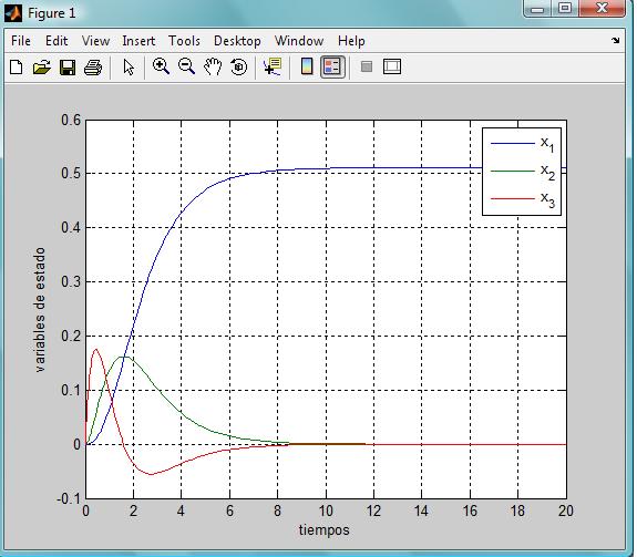
Primero lo haremos para el sistema no lineal.
- Creamos primero la función.
function dx=nolineal(t,x)
R=1; Como nos dice, que simularlo con R=1 y R=5, aqui en la otra simulación simplemente lo cambiamos por 5
dx=zeros(3,1);
dx(1)=x(2);
dx(2)=x(3);
dx(3)=-x(1)-5*x(2)-4*x(3)+R-sin(x(1));
Nota: Al guardar la función, ponerle el mismo nombre que le hemos puesto a la función, en este caso "nolineal"
- Ahora creamos el archivo que va a ejecutar la función.
x0=[0;0;0];
tf=20;
[t,x]=ode45(@nolineal,[0,tf],x0);
plot(t,x),grid
xlabel('tiempos');
ylabel('variables de estado')
legend ('x_1','x_2','x_3')
Y la gráfica que nos devuelve el sistema es
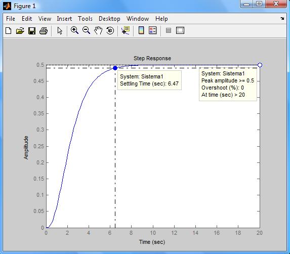
Ahora lo haremos para el sistema lineal
clc, clear all, close all
A=[0,1,0;0,0,1;-2,-5,-4];
B=[0;0;1];
C=[1,0,0];
D=[0];
Sistema1=ss(A,B,C,D); %Coje las 4 matrices y lo convierte en un sistema lineal
step(Sistema1,20)
Y la gráfica que nos devuelve el sistema es
- Versión para imprimir
- Inicie sesión para enviar comentarios
Contenidos licenciados bajo Creative Commons by-sa 3.0

![]()